What’s really going on in PBjam - an advanced tutorial

Introduction

In this example we will demonstrate what is happening under the hood of PBjam. As such this consititutes an advanced tutorial that relies somewhat on basic knowledge of solar-like peakbagging and its terminology. There are many resouces in the scientific literature if the user requires more background (Davies 2016, Basu & Chaplin).

This example will look at a high signal-to-noise ratio red giant with nearly 4 years of high quality Kepler data (KIC 4448777). We will use the Lightkurve tool to handle the data and refer the user to the Lightkurve docs for details and functionality.

import pbjam as pb
import lightkurve as lk
import warnings
warnings.simplefilter("ignore")
print(f'PBjam version == {pb.__version__}')

2021-05-05, 07:59:22 - theano.tensor.blas: Using NumPy C-API based implementation for BLAS functions.
2021-05-05, 07:59:22 - theano.tensor.blas: Using NumPy C-API based implementation for BLAS functions.

PBjam version == 1.0.1

KIC 4448777 has already been extensively studied and the interested reader can find more here. Table 2 of this work lists mode frequencies that we can use as a comparison with our results later.

Setup

We start by setting up the exisiting knowledge of the star. We take literature values of \(\nu_{\rm max}\), \(\Delta {\nu}\), Teff, and Gaia \(G_{\rm bp} - G_{\rm rp}\). Each observable is set up as a tuple in the form (value, uncertainty).

kic = '4448777'
numax = (220.0, 3.0)  # in microhertz
dnu = (16.97, 0.05)   # in microhertz
teff = (4750, 250)    # in Kelvin
bp_rp = (1.34, 0.1)   # in mag

Data collection and preparation

We handle all of our data in this tutorial using lightkurve. First we download all available lightcurves:

lcs = lk.search_lightcurve(kic, exptime=1800, mission='Kepler').download_all()

We then process the lightcurve collection by concatenating, normalizing, flattening, and the finally removing outliers:

lc = lcs.stitch().normalize().flatten(window_length=401).remove_outliers(4)

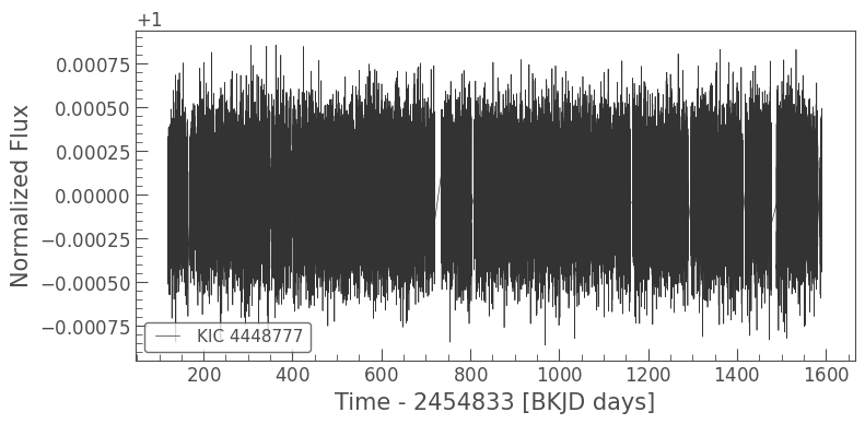
Lightkurve provides plot functionality for its lightcurve objects and so to plot the time series data we simply:

lc.plot();

We then use the Lightkurve periodogram functionality to get a critically sampled power spectrum with frequency units of \(\mu \rm Hz\) (i.e., normalization=’psd’). We set the maximum and minimum frequency of the periodogram based on the estimated numax and dnu and finally we flatten the periodogram.

The flatten function uses Lightkurve’s inbuilt method to remove the broadband background power but maintains the modes of oscillation. The Lightkurve method uses a simple estimation of the background based on a varying width median filter in log space, and divides the power by the estimated background to produce what is commonly referred to as a signal-to-noise spectrum. The Lightkurve implementation is less than optimal but fast and easy to use. If you care about the treatment of the background and worry about its impact on your results then you can implement your own method here (for example background fitting) to produce a flattened periodogram.

pg = lc.to_periodogram(normalization='psd',
                      minimum_frequency=numax[0] - dnu[0] * 4,
                      maximum_frequency=numax[0] + dnu[0] * 4).flatten()

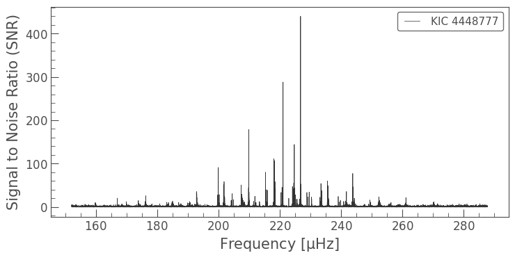
Again, a Lightkurve periodogram has a plot function:

pg.plot()

<matplotlib.axes._subplots.AxesSubplot at 0x7f7e37cfffd0>

At this stage our setup is complete. We have some observed properties and we have some data. We move on to using PBjam to try to understand and interpret the data we have.

PBjam

Motivation

Most of the effort in PBjam (both computational and developmental) is applied to determining mode degree identification given some periodogram. For this task we break up what we know into two components:

\begin{align*} P(M \, | \, D) \propto P(M) \, P(D \, | \, M), \end{align*}

where \(P(M \, | \, D)\) is the posterior probability of some model \(M\) given the data \(D\), \(P(M)\) is the prior constraint on \(M\), and \(P(D \, | \, M)\) is the probability of \(M\) given the data. If we use a more informal syntax then the prior is what we know already, the likelihood tells us what we know from the data, and the posterior is what we care about: the combination of our exisiting knowledge and our new knowledge.

For peakbagging solar-like oscillations we have a wealth of experience and exisiting knowledge. The Kepler mission has provided excllent data sets for thousands of solar-like oscillators. PBjam uses this exisiting data set to generate a prior probability function \(P(M)\). In PBjam we call the kde prior function kde because, well because.

For the likelihood function to provide a model to compare with the data, we use a simple asymptotic relation that describes the well established pattern of radial and quadrupole modes in the periodogram. The pattern is not much more than the sum of regularly spaced Lorentzian profiles in addition to some background. This pattern provides a simple model than can be used as \(M\) and allows for the easy evaluation of \(P(D \, | \, M)\). We use asy_peakbag to estimate \(P(M \, | \, D)\) and hence make a mode identification.

Once mode identification is complete, we perform the actual peakbagging using peakbag. This peakbagging uses a new model and is powered by the NUTS sampler of PyMC3. Here we try to minimise the prior constraints from the previous steps leaking through into the fit. But, there is a trade off between speed and stability vs minimum prior constraint. We will discuss the priors in more detail in the peakbag section.

kde

The prior function we build is a continuous function based on previously fitted solar-like oscillator examples. There are many way of building a prior function but here we use a Kernel Density Estimation (KDE) approach where previous results are used as input.

A KDE is fundamentally a data smoothing problem and many users will be familar with 1D KDE’s. Here we use a multidimensional KDE with a band width for each of the 10 dimensions we implement. This gives full control over the degree of smoothing of the prior data. The KDE is constructed as:

\begin{align*} P(\mathbf x) \propto \frac{1}{n} \sum_{i=1}^{n} {\mathbf K_{\mathbf H}}({\mathbf x - \mathbf x_{i}}), \end{align*}

where \(\mathbf x\) are the input parameters, \(\mathbf x_{i}\) is one of \(n\) prior data points used to construct the prior. \(\mathbf K_{\mathrm H}\) is the band width matrix for which we use a multivariate Gaussian covariance matrix with all off-axis elemets set to zero (sometimes called a D-type kernel):

\begin{align*} {\mathbf K_{\mathbf H}} = (2 \pi)^{-d / 2} |\mathbf H|^{-1/2} \exp \left( -\frac{1}{2} \mathbf x^{T} \mathbf H ^{-1} \mathbf x\right), \end{align*}

where \(d\) is the number of dimensions of the multivariate KDE and we construct \(\mathbf H\) as.

\begin{align*} \mathbf H = {\mathrm{diag}(\mathbf \sigma)} \, \mathbf I \, {\mathrm{diag}(\mathbf \sigma)}, \end{align*}

where \(\mathbf I\) is the \(d \times d\) identity matrix.

As a normalized probability density function it is straight forward, using MCMC sampling tools, to estimate the posterior distribution \(P(M \, | \, D)\) given some set of observations on parameters of the KDE. In kde we use emcee to sample the posterior distribution given some observations.

In PBjam we determine the optimal band width (\(\sigma\)) coefficients using a cross validated maximum likelihood approach. This approach creates a smooth function that is largely insensitive to indivdual data points. The optimal band width will be larger when the density of prior data points less but smaller when we have more data points. As such the prior constraint priorvide by the KDE is expected to improve as we populate the prior with more robust examples of solar-like oscillations. Note, to account for a larger spread in signal-to-noise examples in expected useage compared to the prior data we dramactially increase the band width values of the axis asscoiated with the signal-to-noise ratio.

Background to one side, here is how to run kde. We start with an instance of kde and the call this instance while passing in observables.

K = pb.kde()
K(dnu=dnu, numax=numax, teff=teff, bp_rp=bp_rp)

Steps taken: 2000
Steps taken: 3000
Steps taken: 4000
Steps taken: 5000
Chains reached stationary state after 5000 iterations.

K.samples contains information on the estimated values of the KDE which we will elaborate on later. It is the posterior and its interpretation that is iteresting to us.

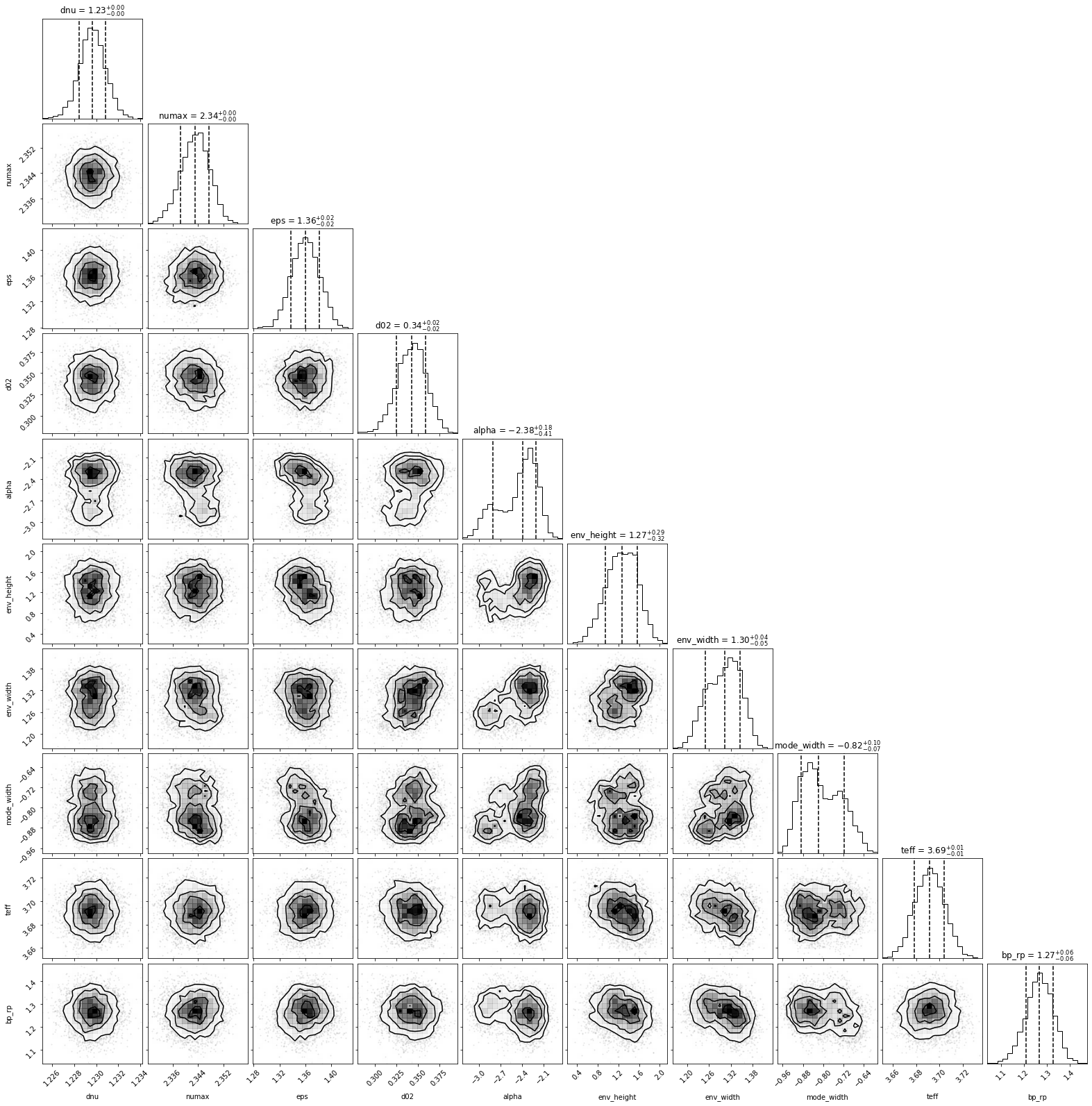
We can plot the corner plot of the posterior using the convience function:

K.plot_corner();

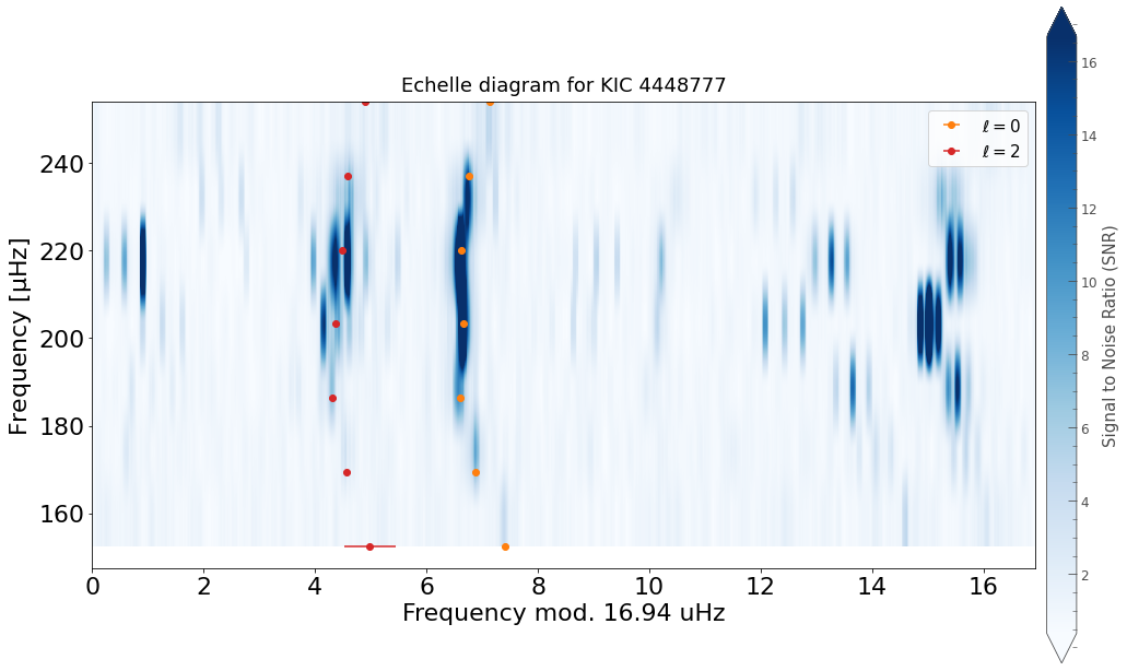
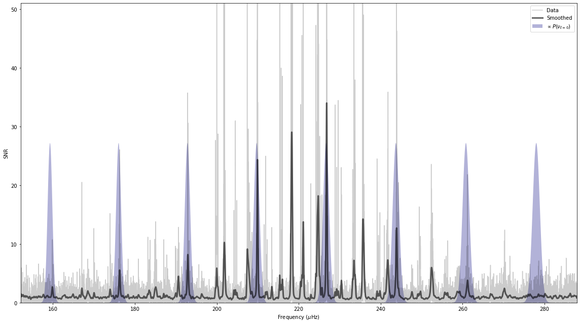
We can also plot the interpretation of the posterior. Given the posterior distribution, we can predict the location in frequency of the \(\ell = 0\) modes, which we label as \(P(\nu_{\ell=0})\). The plot method of the kde class can be called with a Lightkurve periodogram as the only argument, and this will display the distribution of the prediction of the location in frequency of the \(\ell = 0\) modes in navy blue.

K.plot_spectrum(pg);

asy_peakbag

At this point we are ready to introduce the constraint from our data. We estimate \(P(M \, | \, D)\) using the prior from kde. For the likelihood function we fit an asymptotic approximation of a series of radial and quadrupole modes.

The model is built with Lorentzian profiles to model modes of oscaillations as damped harmonic oscillators:

\begin{align*} \mathcal{L}(\nu \, | \, \nu_{0}, w, h) = \frac{h} {(1.0 + \frac{4.0}{w^2} (\nu - \nu_{0})^2)}, \end{align*}

where $ \nu_{0}$ is the mode central frequency, \(w\) is the mode line width, and \(h\) is the mode height. The model then is:

\begin{align*} M (\nu) = 1.0 + \sum_{n} \left( \mathcal{L}(\nu \, | \, \nu_{n, \ell=0}, w_{n, \ell=0}, h_{n, \ell=0}) + \mathcal{L}(\nu \, | \, \nu_{n, \ell=2}, w_{n, \ell=2}, h_{n, \ell=2}) \right). \end{align*}

Rather than fitting a series of free parameters for each mode we use some deterministic relations to encode what we believe we know about the mode pattern in solar-like oscillators. Each mode frequency is determined with:

\begin{align*} \nu_{n, \ell=0} = (n + \epsilon + \frac{\alpha}{2}(n - n_{\mathrm{max}})^2)\Delta \nu , \end{align*}

where \(\epsilon\) is commonly referred to as an offset, or even phase, term, \(\alpha\) is a curvature term, and \(n_{\mathrm max} = \nu_{\mathrm{max}} / \Delta \nu - \epsilon\).

Quadrupole modes are offset from the radial modes by \(d_{02}\):

\begin{align*} \nu_{n, \ell=2} = \nu_{n, \ell=0} - d_{02}. \end{align*}

Modes heights are determined using a Gaussian envelope where,

\begin{align*} h_{n, \ell=0} = H_{\mathrm{max}} \exp \left( - 0.5 \, \frac{(\nu - \nu_{\mathrm{max}})^2}{W_{\mathrm{env}}^2} \right) \end{align*}

where \(W_{\mathrm{env}}\) is the mode envelope width, and \(H_{\mathrm{max}}\) is the mode envelope height. We set \(h_{n, \ell=2} = 0.7 \, h_{n, \ell=0}\).

For mode line width we use a single value for all modes which is an over simplication but helps keep the model as simple as possible.

We use the emcee code to estimate the posterior probability distribution. Note, while above in the kde class we passed in all of \(\nu_{\rm max}\), \(\Delta {\nu}\), Teff, and Gaia \(G_{\rm bp} - G_{\rm rp}\), here we use only Teff, and Gaia \(G_{\rm bp} - G_{\rm rp}\) in order to prevent over constraining the \(\nu_{\rm max}\), \(\Delta {\nu}\) parameters that have most likely been determined using the same data sets as we are using here. We use the results from the kde run above to set the starting parameters for emcee.

First we’ll create a star class instance and attach the results from the KDE.

st = pb.star(kic, pg, numax, dnu, teff, bp_rp)
st.kde = K

And here is how we run asy_peakbag:

pb.asy_peakbag.asymptotic_fit(st, norders=7);
st.asy_fit('cpnest', developer_mode=False);

2021-05-05, 08:02:48 - CPNest  : Running with 1 parallel threads
2021-05-05, 08:08:54 - CPNest  : Final evidence: -22927.33
2021-05-05, 08:08:54 - CPNest  : Information: 20.93
2021-05-05, 08:08:54 - CPNest  : Sampler process 105310: MCMC samples accumulated = 0
2021-05-05, 08:08:54 - CPNest  : Sampler process 105310 - mean acceptance 0.185: exiting
2021-05-05, 08:08:55 - CPNest  : Computed log_evidences: (-22927.436606695235,)
2021-05-05, 08:08:55 - CPNest  : Relative weights of input files: [1.0]
2021-05-05, 08:08:55 - CPNest  : Relative weights of input files taking into account their length: [1.0]
2021-05-05, 08:08:55 - CPNest  : Number of input samples: [2883]
2021-05-05, 08:08:55 - CPNest  : Expected number of samples from each input file [511]
2021-05-05, 08:08:55 - CPNest  : Samples produced: 511
2021-05-05, 08:08:57 - CPNest  : Computed log_evidences: (-22927.436606695235,)
2021-05-05, 08:08:57 - CPNest  : Relative weights of input files: [1.0]
2021-05-05, 08:08:57 - CPNest  : Relative weights of input files taking into account their length: [1.0]
2021-05-05, 08:08:57 - CPNest  : Number of input samples: [2883]
2021-05-05, 08:08:57 - CPNest  : Expected number of samples from each input file [552]
2021-05-05, 08:08:57 - CPNest  : Samples produced: 552

where the arguments are the star class instance from above and the number of radial orders to fit.

We can plot the model for the starting parameters to see if we have reasonable starting values:

In this case, the starting values are very close to the what we would anticipate as the final values. This happens even though KIC 4448777 is not included in the prior data. We can then proceed and run the asymptotic fit.

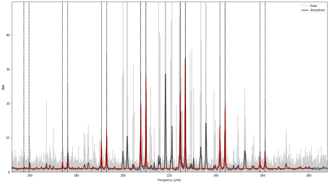
As in kde, asy_peakbag has plot_spectrum and plot_corner functions.

st.asy_fit.plot_spectrum();

st.asy_fit.plot_corner();

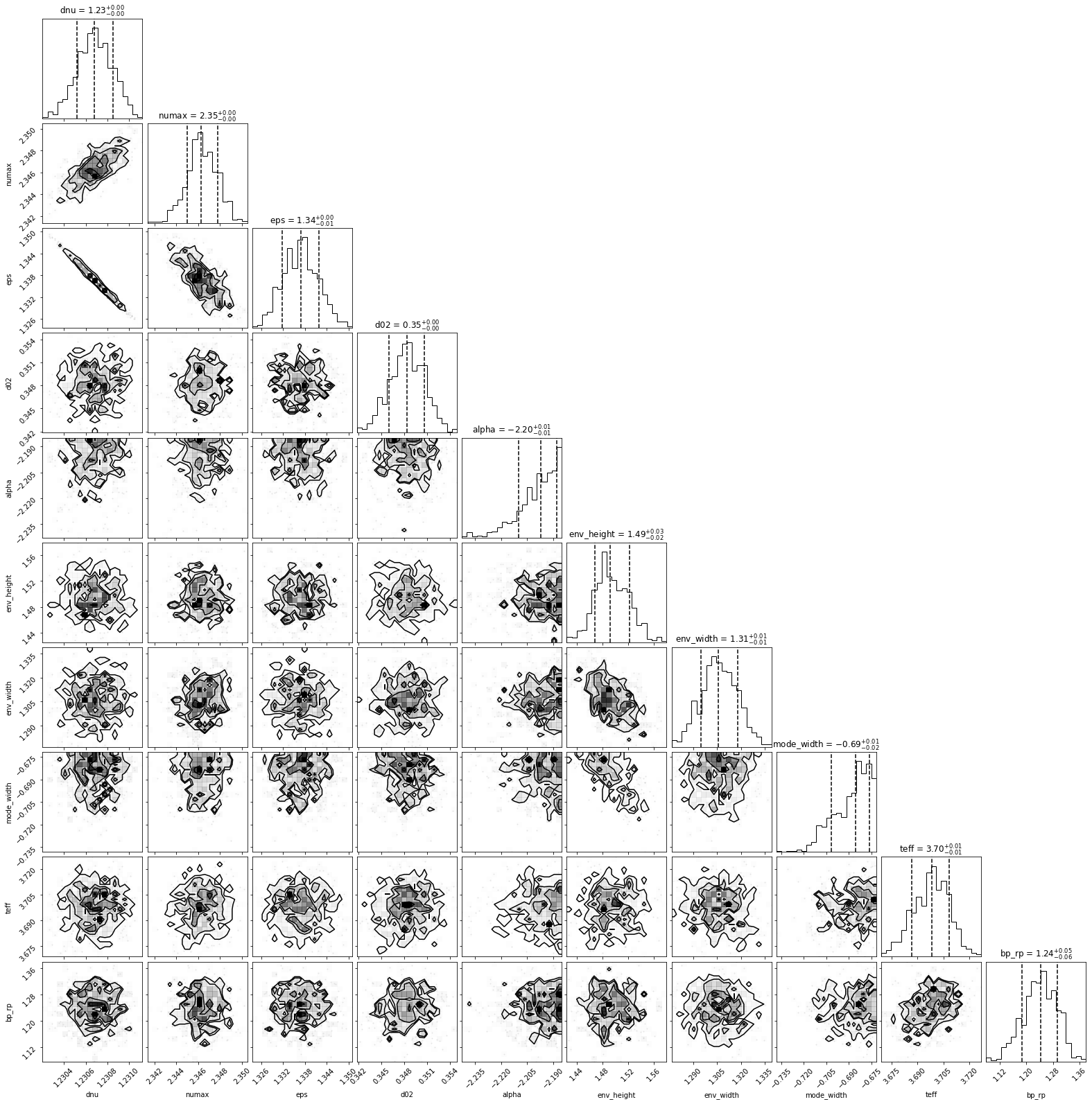
If we are happy with the mode identification performed by asy_peakbag we can move on to the actual peakbagging. All the information required for the actual peakbagging is stored in st.asy_fit and st.asy_fit which includes summary statistics for the fitted parameters and the predicted location in frequency of the radial and quadrupole modes.

peakbag

Our actual peakbagging will be performed using PyMC3 and the NUTS (no U-turn sampler). PyMC3 is a probabilistic programming language and so we will adopt consistent notation here. We introduce the following notation:

\begin{align*} Y \sim \mathcal{N}(\mu, \sigma^2), \end{align*}

which in words says we view \(Y\) as a random variable that is distributed according to a normal distribution with mean \(\mu\) and standard deviation \(\sigma\). This notation is extremely useful as it allows us to very nearly mirror the peakbagging code used in peakbag.

peakbag has at least two peakbagging models, and more will be added as we develop, but the basic example is called the 'simple' model. In this model we keep all parameters as independent of each other as possible.

We start our description by considering just the radial mode frequencies. Given the results of asy_peakbag we have reliable predictions of where the radial modes are located in frequency. This allows us to set up random variables to describe the radial mode frequencies. The distribution we chose as the prior on the radial mode frequencies is the normal distribution, with the mean as the prediction from asy_peakbag and the standard deviation as 3% of \(\Delta \nu\). Using the notation above, for each \(n\), the prior on the mode frequencies can be written as:

\begin{align*} \nu_{n, \ell=0} \sim \mathcal{N}(\nu_{n, \ell=0, \mathrm{pred}}, (0.03 \, \Delta \nu)^2) \end{align*}

If we were to turn this statement into a PyMC3 model and perform sampling, we would get posterior distributions that we normally distributed with the means as the predicitons and the standard deviations as \(3\%\) of \(\Delta \nu\). We will continue to construct priors for all our parameters. Quadrupole modes follow the same for as radial modes.

\begin{align*} \nu_{n, \ell=2} \sim \mathcal{N}(\nu_{n, \ell=2, \mathrm{pred}}, (0.03 \, \Delta \nu)^2). \end{align*}

Mode line widths are parameters that can only take positive values. In order to encode our prior knowledge and to keep line widths positive we use a log normal distribution. As the prior mean value for line width we use the line width estimated in asy_peakbag. As a standard deviation we use \(1.0\) in log space which corresponds to a \(270\%\) uncertainty in non-log space. We write this as:

\begin{align*} w_{n, \ell=0} \sim \mathrm{Log\mathcal{N}}(\log w_{\mathrm{pred}}, 1.0), \end{align*}

and

\begin{align*} w_{n, \ell=2} \sim \mathrm{Log\mathcal{N}}(\log w_{\mathrm{pred}}, 1.0). \end{align*}

We use the same arrangement for mode heights. Here we use a smaller standard deviation of \(\sim 50\%\) to reflect our improved confidence in the mode height predictions.

\begin{align*} h_{n, \ell=0} \sim \mathrm{Log\mathcal{N}}(\log h_{n, \ell=0, \mathrm{pred}}, 0.4^2), \end{align*}

and

\begin{align*} h_{n, \ell=2} \sim \mathrm{Log\mathcal{N}}(\log h_{n, \ell=2, \mathrm{pred}}, 0.4^2). \end{align*}

Finally we construct a prior for the background component. As we are working with flattened periodograms the background in a perfect world would be unity. However, the flattening becomes an increasingly bad approximation as the signal-to-noise ratio of the modes becomes high. Fortunately, in the high SNR case this has only a small effect on peakbagging results. However, to provide a more robust result we allow the background around pairs of modes to vary as a function of order. We setup the prior as :

\begin{align*} b_{n} \sim \mathrm{Log\mathcal{N}}(\log 1.0, 0.4^2). \end{align*}

With the prior constructed and all parameters of the simple model defined we can calculate the model. Using short hand notation with \(\mathcal{L}(\nu, n, \ell)\) representing a Lorentzian profile for mode \(n, \ell\), we define the peakbagging model \(M\) as:

\begin{align*} M_{n} (\nu) = b_{n} + \mathcal{L}(\nu, n, \ell=0) + \mathcal{L}(\nu, n, \ell=2). \end{align*}

In the final step of building our PyMC3 model we think of the observed data as being random variables drawn from some distribution. The noise characterisitics of periodograms are typically \(\chi^{2}\) with 2 degrees of freedom. In our case as we are using a flattened periodogram we have to account for the differences in mean values from the \(\chi^{2}\) with 2 degrees of freedom distribution (which is 2) and the observed data which is 1 because of the way we prepared the data. This is easy to do in PyMC3.

The \(\chi^{2}\) with 2 degrees of freedom distribution is a special case of the gamma distribution. Taking into account the different means, the flattened periodogram should be gamma distributed with \(\alpha = 1\) and \(\beta = \frac{1}{M(\nu)}\). We write this as:

\begin{align*} D \sim \mathcal{\Gamma}(1, \frac{1}{M(\nu)}), \end{align*}

where \(D\) is the observed data - the flattend periodogram. And then our PyMC3 model is constructed. We use the NUTS sampler to draw samples from the posterior probability distribution.

All of the above functionality can be called with the following code:

%%time
pb.peakbag(st)
st.peakbag(model_type='simple', nthreads=4, tune=1500)

2021-05-05, 08:09:24 - pymc3   : Auto-assigning NUTS sampler...
2021-05-05, 08:09:24 - pymc3   : Initializing NUTS using adapt_diag...
2021-05-05, 08:09:32 - pymc3   : Multiprocess sampling (4 chains in 4 jobs)
2021-05-05, 08:09:32 - pymc3   : NUTS: [back, height2, height0, l2, l0, width2, width0]
2021-05-05, 08:13:48 - pymc3   : Sampling 4 chains for 1_500 tune and 1_000 draw iterations (6_000 + 4_000 draws total) took 256 seconds.

CPU times: user 1min 11s, sys: 19.2 s, total: 1min 30s
Wall time: 4min 57s

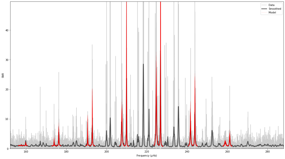
We can inspect the results by looking at the data with models built from samples of the posterior over plotted. The easiest way to do this is to call the plot_spectrum() function.

st.peakbag.plot_spectrum();

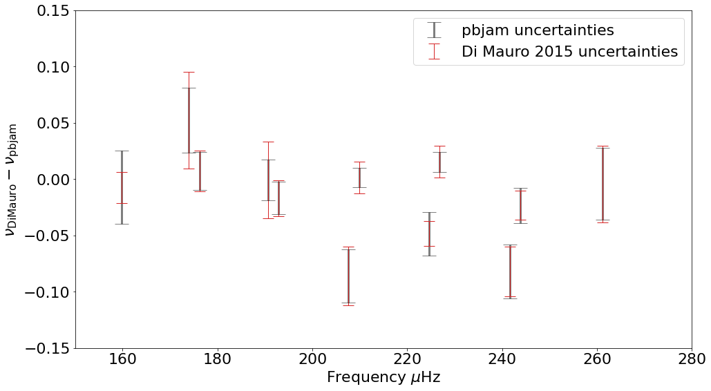
Comparison with published values

We can check our results against published values for consistency. We use the values from Di Mauro, 2015.

DiMauro_l0 = [159.842,  176.277,  192.907, 209.929, 226.831,  243.879,  261.215]
DiMauro_l0_unc = [0.014, 0.018, 0.016, 0.014, 0.014, 0.013, 0.034]
DiMauro_l2 = [0, 174.005, 190.623, 207.551, 224.646,  241.630, 0]
DiMauro_l2_unc = [0, 0.043, 0.034, 0.026, 0.011, 0.022, 0]

norders = st.peakbag.norders
pbjam_mean_l0 = st.peakbag.samples[:,:norders].mean(axis=0)
pbjam_std_l0 = st.peakbag.samples[:,:norders].std(axis=0)
pbjam_mean_l2 = st.peakbag.samples[:,norders:2*norders].mean(axis=0)
pbjam_std_l2 = st.peakbag.samples[:,norders:2*norders].std(axis=0)

import matplotlib
import matplotlib.pyplot as plt
matplotlib.rcParams.update({'font.size': 22})
fig, ax = plt.subplots(figsize=[16,9])
ax.errorbar(DiMauro_l0, DiMauro_l0 - pbjam_mean_l0, yerr=pbjam_std_l0, label='pbjam uncertainties',
            fmt='k-', barsabove=True, linestyle='none', alpha=0.5, capsize=10, elinewidth=3)

ax.errorbar(DiMauro_l0, DiMauro_l0 - pbjam_mean_l0, yerr=DiMauro_l0_unc, label='Di Mauro 2015 uncertainties',
            fmt='C3-', barsabove=True, linestyle='none', capsize=8, elinewidth=1)

ax.errorbar(DiMauro_l2, DiMauro_l2 - pbjam_mean_l2, yerr=pbjam_std_l2, fmt='k-', barsabove=True,
            linestyle='none', alpha=0.5, capsize=10, elinewidth=3)

ax.errorbar(DiMauro_l2, DiMauro_l2 - pbjam_mean_l2, yerr=DiMauro_l2_unc, fmt='C3-', barsabove=True,
            linestyle='none', capsize=8,elinewidth=1)
ax.set_ylim([-.15,0.15])
ax.set_xlim([150, 280])
ax.legend()
ax.set_xlabel(r'Frequency $\mu \rm Hz$')
ax.set_ylabel(r'$\nu_{\rm Di Mauro} - \nu_{\rm pbjam}$')

Text(0, 0.5, '$\\nu_{\\rm Di Mauro} - \\nu_{\\rm pbjam}$')

st.peakbag.plot_echelle();